Программные продукты и системы

Introduction. Applied Quantum  Search Algorithm Model

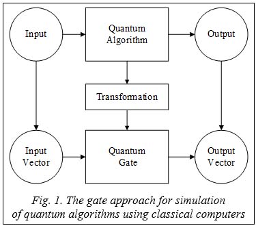
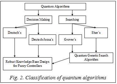
Grover Quantum Search Algorithm (QSA) is one of the famous quantum algorithms (QA) that outperform their classical counterparts [1–4].  In the conventional linear search algorithm, it required  comparisons to find an element in an array of length N. Grover’s algorithm achieves a quadratic speed up; i.e., it has a complexity of  Grover’s search algorithm provides an example of the speed-up that would be offered by quantum computers (if and when they are built) and has the important application in solution of global optimization control problems. The problem solved by Grover’s algorithm is finding a sought-after ("marked ") element in an unsorted database (DB) of size N. To solve this problem,  a classical computer would need  database queries on average, and in the worst case it would N –1 queries.

Thus, using Grover’s algorithm, a quantum computer can find the marked state using only  quantum data queries. In the case of M "marked " elements in an unsorted DB of size N speed-up of quantum search process increases as . It is believed that this complexity is optimal. This speed up is inherently due to the parallel computational nature of quantum operators that can affect all of the coefficients in the state expansion at once.

General design structure  of quantum algorithms

A quantum algorithm calculates the qualitative properties of the function f.

From a mathematical standpoint, a function f  is the map of one logical state into another.

The problems solved by a QA can be stated as follows:

Given a function f :{0,1}n®{0,1}m; find a certain property of the function f.

Or in the symbolic form as:

Input: A function f :{0,1}n®{0,1}m.

Problem: Find a certain property of f.

Figure 1 is a block diagram showing a gate approach for simulation of a QA using classical computers [5]:

In Fig. 1, an input is provided to a QA and the QA produces an output. However, the QA can be transformed to produce a quantum algorithmic gate (QAG) such that an input vector (correspond- ing to the QA input) is provided to the QAG to produce an output vector (corresponding to the QA output) [5].

Figure 2 shows classification tree of QA’s for quantum soft computing and control engineering applications. QA’s are either decision-making or searching as described above.

As shown, as example, in Fig. 2, Quantum Genetic Search Algorithms (QGSA) follows from Grover’s and Shor’s algorithms, and background for Robust KB design of Fuzzy Controllers follows from Deutch’s, Deutch–Josa’s, Grover’s and/or Shor’s algorithms (see in details [4, 5]).

Let us briefly consider the design process of QAG.

Figure 3 is a block diagram showing the design process of the QAG.

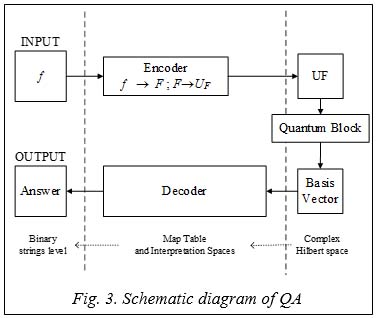
In Fig. 3 an input block of the QA is a function f that maps binary strings into binary strings. This function f is represented as a map table, defined for every string its image. The function is first encoded into a unitary matrix operator UF depending on the properties of f. In some sense, this operator calculates f when its input and output strings are encoded into canonical basis vectors of a complex Hilbert space. The operator UF maps the vector code of every string into the vector code of its image by f. The quantum block operates on basis vectors in a complex Hilbert space. The vectors operated on by the quantum block are provided to a decoder, which decodes the vectors to produce an answer.

Once generated, the matrix operator UF  is embedded into a quantum gate G. The quantum gate G is a unitary matrix whose structure depends on the form of matrix UF  and on the problem to be solved. The quantum gate is a unitary operator built from the dot composition of other more specific operators. The specific operators are described as tensor products of smaller matrices.

General structure of the  QAG design method

Traditionally QA is written as a quantum circuit [2].

Figure 4 shows the general structure of a quantum circuit for a QAG.

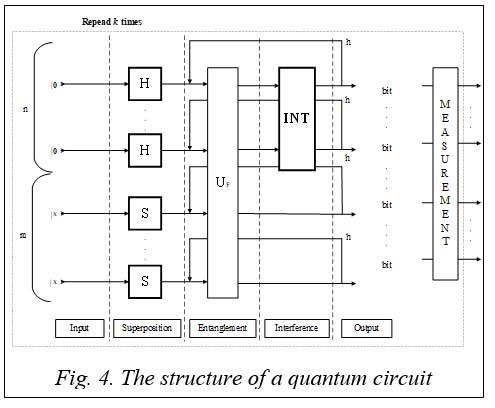
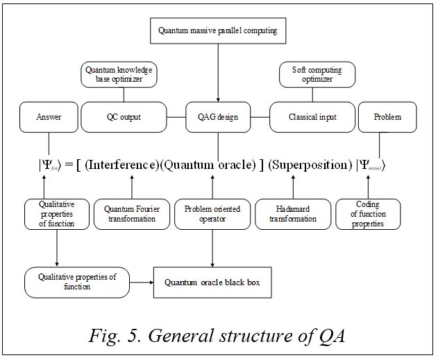
As shown in Fig. 4, the general structure of the quantum circuit is based on three reversible quantum operators (superposition, entanglement, and interference) and irreversible classical operator measurement.

The quantum circuit is a high-level description of how these smaller matrices are composed using tensor and dot products in order to generate the  final quantum gate as shown in Fig. 4 (see in details [4, 5]). Thus, the mathematical background of this approach is based on mappings between the quantum block operations in the complex Hilbert space [2].

The encoder and decoder operate in a map table and interpretation space, and input/output occurs on a binary string level. The Clifford and Pauli groups are the background for universal QAG design for simulation of a QA’s on classical computers. Therefore, the general structure of the QAG is based on three quantum operators as superposition, entanglement, and interference, and measurement is irreversible classical operation.

The QAG acts on an initial canonical basis vector to generate a complex linear combination (called a superposition) of basis vectors as an output. This superposition contains the full information to answer the initial problem. After the superposition has been created, measurement takes place in order to extract the answer information.  In quantum mechanics, a measurement is a non-deterministic operation that produces as output only one of the basis vectors in the entering superposition. The probability of every basis vector of being the output of measurement depends on its complex coefficient (probability amplitude) in the entering complex linear combination.

Thus, the segmental action of the quantum gate and of measurement makes up a quantum block (see Fig. 3). The quantum block is repeated k times in order to produce a collection of k basis vectors. Since measurement is a non-deterministic operation, these basis vectors will not necessarily be identical, and each basis vector encodes a piece of the information needed to solve the problem. The last part of the algorithm involves interpretation of the collected basis vectors in order to get the final answer for the initial problem with some probability.

Peculiarities of general QA-structure

As mentioned above, QA estimates (without numerical computing) the qualitative properties of the function f. From a mathematical standpoint, a function f is the map of one logical state into another. The problem solved by a QA can be stated in the symbolic form as follows:

Find a certain property of function f that is a map f:{0,1}n ®{0,1}m.

Main goal of QA applications is the study and search of qualitative properties of functions as the solution of problem. Figure 5 shows the general structure of QA.

The main blocks in Fig. 5 are following: i) unified operators; ii) problem-oriented operators; iii) Benchmarks of QA simulation on classical computers; and iv) quantum control algorithms based on quantum fuzzy inference (QFI) and QGA as new types of QSA. The design process of QAG’s includes the matrix design form of three quantum operators: superposition (Sup), entanglement (UF) – oracle, and interference (Int) that are the background of QA structures.

In general form, the structure of a QAG for QA in Fig. 5 can be [5] described as follows:

     (1)

where I is the identity operator; the symbol Ä denotes the tensor product; S is equal to I or H and dependent on the problem description. The heart of the quantum block is the quantum gate, which depends on the properties of matrix UF. One portion of the design process in Eq. (1) is the type-choice of the entanglement problem dependent operator UF that physically describes the qualitative properties of the function f.

A general QA, written as a quantum circuit  (as in Fig. 4), can be automatically translated into the corresponding programmable quantum gate for efficient classical simulation. This gate is represented as a quantum operator in matrix form such that, when it is applied to the vector input representation of the quantum register state, the result is the vector representation of the desired register output state.

Main QAG’s and main quantum operators

Three quantum operators, superposition, entanglement (quantum oracle), and interference, are the basis for quantum computations of qualitative and quantitative measures in quantum soft computing.

As described above (see Fig. 3) the structure of a QAG based on these three quantum operations of superposition, entanglement, and interference. Thus, superposition, entanglement (quantum oracle) and interference in quantum massive parallel computing are the main operators in QA. The superposition operator of most QA’s can be expressed as following: , where n and m are the numbers of inputs and of outputs respectively. Operator S may be or Hadamard operator H or identity operator I depending on the algorithm. Numbers of outputs n as well as structures of corresponding superposition and interference operators are presented in the Table 1 for different QA’s on Fig. 2.

Table 1

Parameters of superposition and interference  operators of main QA

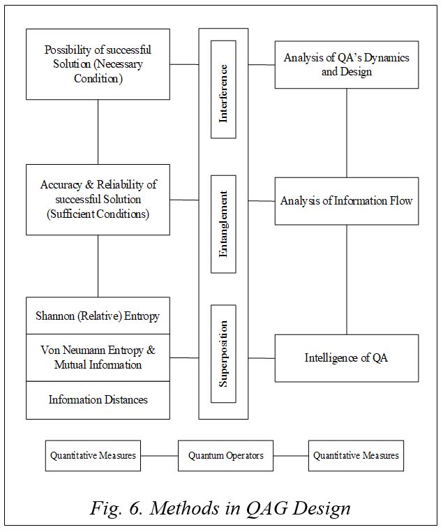
Figure 6 shows methods in QAG design. The methods as shown in Fig. 6 are based on qualitative measures of QAG design: 1) analysis of QA dynamics and structure gate design; 2) analysis of information flow; and 3) structure simulation of intelligent QA’s on classical computers.

Remark. The analysis of information flow  in [4, 5] is described. In this article analysis of QA dynamics and structure gate design, and structure simulation of intelligent QA’s on classical computers are discussed.

As shown in Fig. 6 analysis of QA dynamics provides the background for showing the existence of a solution and that the solution is unique with the desired probability. Analysis of information flow in the QA gates provides the background for showing that the unique solution exists with the desired accuracy and that the reliability of the solution can be achieved with higher probability.

The intelligence of a QA is achieved through the principle of minimum information distance between Shannon and von Neumann entropy and includes the solution of the QA stopping problem (see [5]). The output states of a QA as the solution of expected problems are the intelligent states with minimum entropic relations of uncertainty (coherent superposition states). The successful results of QA computing are robust to noise excitations in quantum gates, and intelligent quantum operations are fault-tolerant in quantum soft computing [5].

With the method of quantum gate design presented herein, various different structures of QA can be realized (see Fig. 4), as shown in Table 2 below.

Remark. A quantum computer is difficult to build because of decoherence effects. Decoherence introduces errors in the superposition. The decoherence problem is reduced by using tools of quantum soft computing such as a QGSA. Errors produced by decoherence are of three kinds: (i) phase errors; (ii) bit-flip errors; and (iii) both phase and bit-flip errors.

These three errors can all be modeled using unitary transformations [5].

This means that if the QGSA is implemented on a physical quantum-mechanical system, one would gain the advantages of quantum parallelism and reduce the problem of decoherence, because decoherence can be used as a natural generator of mutation and crossover operators.

Let us discuss briefly any mathematical backgrounds and its physical peculiarities for quantum computing based on QAG.

Design technology of and QAG simulation system

The searching problem can be stated in terms of a list  with a number N of unsorted elements. Denote by x0 the marked element in  that are sought. The quantum mechanical solution of this searching problem goes through the preparation of a quantum register in a quantum computer to store the N items of the list. This will allow exploiting quantum parallelism. Thus, assume that the quantum registers are made of n source qubits so that N = 2n.

A target qubit is used to store the output of function evaluations or calls. To implement the quantum search, construct a unitary operation that discriminates between the marked item x0 and the rest. The following function:

,                              (2)

and its corresponding unitary operation  . It is assumed the access to f via the following quantum oracle: Uf |0,0ñ = |0, f(0)ñ, Uf |1,0ñ = |0, f(1)ñ.

After these two queries, we can measure qubit 1 with a deterministic outcome, and answer whether f(0) =  = f(1). However, a quantum checker can apply Uf  to a linear combination of states in the computational basis. Count how many applications of this operation or oracle calls are needed to find the item. The rationale behind the Grover algorithm is: 1) to start with a quantum register in a state where the computational basis states are equally present; 2) to apply several unitary transformations to produce an outcome state in which the probability of catching the marked state |x0ñ is large enough.

Let's imagine the stages of Gruver's algorithm:

Step 1. Initialize the quantum registers to the state:

        (3)

Step 2. Apply bit-wise the Hadamard one-qubit gate to the source register, so as to produce a uniform superposition of basis states in the source register, and also to the target register:

  (4)

Step 3. Apply the operator :

Let  be the operator by

,  (5)

that is, it flips the amplitude of the marked state leaving the remaining source basis states unchanged.  The state in the source register of Step 3 equals precisely the result of the action of , i.e., |y3ñ = .

Step 4. Apply next the operation D known as inversion about the average. This operator is defined as follows

,

and

where  is the operator in Step 3 for x0 = 0. The effect of this operator on the source is to transform

,                          (6)

where  is the mean of the amplitudes, so its net effect is to amplify the amplitude of |x0ñ over the rest.

Step 5. Iterate Steps 3 and 4 a number of times m.

Step 6. Measure the source qubits (in the computational basis). The number m is determined such that the probability of finding the searched item x0 is maximal.

According to Steps 2–4 above and (1), the QAG of Grover’s QSA is  that acts on the initial state of both registers in the QSA.

Computational analysis of Grover’s QSA is similar to analysis of the Deutsch–Jozsa QA. The basic component of the algorithm is the quantum operation encoded in Steps 3 and 4, which is repeatedly applied to the uniform state |y2ñ in order to find the marked element. Steps 5 and 6 in Grover’s algorithm are also applied in Shor’s QSA. Although this procedure resembles the classical strategy, Grover’s operation enhances by constructive interference of quantum amplitudes the presence of the marked state.

Computational models of QSA

We have considered in [4] five practical approaches to design fast algorithms for the simulation most of known QA’s on classical computers:

1.    Matrix based approach;

2.    Model representations of quantum operators in fast QA’s;

3.    Algorithmic based approach, when matrix elements are calculated on “demand”;

4.    Problem-oriented approach, where we succeeded to run Grover’s algorithm with up to 64 and more qubits with Shannon entropy calculation  (up to 1024 without termination condition);

5.    Quantum algorithms with reduced number of operators (entanglement-free QA, and so on).

Detail description of these approaches is given in [4].

Figure 7 shows the structure description of the QA Benchmark Block.

The efficient implementations of a number of operations for quantum computation include controlled phase adjustment of the amplitudes in the superposition, permutation, approximation of transformations and generalizations of the phase adjustments to block matrix transformations. These operations generalize those used as example in QSA’s that can be realized on a classical computer. The application of this approach is applied herein to the efficient simulation on classical com- puters of the Deutsch QA, the Deutsch–Jozsa QA, the Simon QA, the Shor QA and the Grover QA.

Implementation of a QA is based on a QAG.  In the language of classical computing, a quantum computer is programmed by designing a QAG. The prior art reports relatively few such gates because the basic principles underlying the quantum version of programming are in their infancy and algorithms to date have been programmed by ad-hoc techniques.

The problems solved by the QA can be stated as follows:

Input: A function f :{0,1}n®{0,1}m.

Problem: Find a certain property of f.

The structure of a quantum operator Uf  in QA’s as shown in block of Fig. 3 is outlined, with a high-level representation, in the scheme diagram Fig. 1. In Fig. 3 the input of the QA is a function f that maps from binary strings into binary strings. This function is represented as a map table, defining for every string its image. The function f is encoded according to an F – truth table. The function is transformed according to a transform Uf  – truth table into a unitary matrix operator Uf  depending on f’s properties. In some sense, this operator calculates f when its input and output strings are encoded into canonical basis vectors of a complex Hilbert space: Uf  maps the vector code of every string into the vector code of its image by f.  A squared matrix Uf  on the complex field is unitary if and only if (iff) its inverse matrix coincides with its conjugate transpose: A unitary matrix is always reversible and preserves the norm of vectors.

Figure 8 shows structure of the quantum block from Fig. 3.

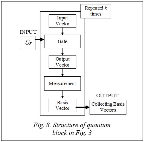
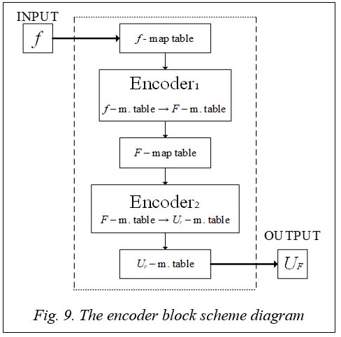
In the structure, the matrix operator UF has been generated it is embedded into a quantum gate as a QAG, a unitary matrix whose structure depends on the form of matrix UF and on the problem to be solved. In the QA, the QAG acts on an initial canonical basis vector (which can always choose the same vector) in order to generate a complex linear combination (superposition) of basis vectors as output. This superposition contains all the information to answer the initial problem.

After this superposition has been created, in measurement block takes place in order to extract this information. In quantum mechanics, measurement is a non-deterministic operation that produces as output only one of the basis vectors in the entering superposition. The probability of every basis vector of being the output of measurement depends on its complex coefficient (probability  amplitude) in the entering complex linear combination.

The segmental action of the QAG and of measurement characterizes the quantum block in Fig. 8. The quantum block is repeated k times in order to produce a collection of k basis vectors. Since measurement a nondeterministic operation, these basic vectors are not be necessarily identical and each one of them will encode a piece of the information needed to solve the problem. The collection block in Fig. 8 of the algorithm outputs the interpretation of the collected basis vectors in order to get the answer for the initial problem with a certain probability.

Encoder

The behavior of the encoder in Fig. 3 is described in the scheme diagram of Fig. 9.

Function f is encoded into matrix UF in three steps.

In step 1, the map table (f – truth table) of function f :{0,1}n®{0,1}m is transformed into the map table (F – truth table) of the injective function F :{0,1}n+m®{0,1}n+m such that:

Remark. The need to deal with an injective function comes from the requirement that UF is unitary. A unitary operator is reversible, so it cannot map two different inputs in the same output. Since UF will be the matrix representation of F, F is injective. If one directly employed the matrix representation of function f, one could obtain a non-unitary matrix, since f could be non-injective. So, injectivity is fulfilled by increasing the number of bits and considering function F instead of function f. The function f can be calculated from F by putting (y0, …, ym–1) = (0, …, 0) in the input string and reading the last m values of the output string.

Reversible circuits realize permutation operations. It is possible to realize any Boolean circuit by reversible circuit. For this case, one need not calculate the function . One can calculate another function with expanding  that is defined as following relation:  where the operation Ä is defined as addition on module 2.

Then the value of F(x) is defined as . For example, the XOR operator between two binary strings p and q of length m is a string s of length m such that the i-th digit of s is calculated as the exclusive OR between the i-th digits of p and q:

In step 2, the function from F map table is transformed into Uf  map table, according to the following constraint:

                                                                       (7)

The code map

 is such that:

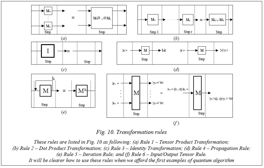
Code t maps bit values into complex vectors of dimension 2 belonging to the canonical basis  of . Besides, using tensor product, t maps the general state of a binary string of dimension n into a vector of dimension 2n, reducing this state to the joint state of the n bits composing the register. Every bit state is transformed into the corresponding 2-dimesional basis vector and then the string state is mapped into the corresponding 2n-dime- sional basis vector by composing all bit-vectors through tensor product. In this sense tensor product is the vector counterpart of state conjunction. Basis vectors are denoted using the ket notation |iñ. This notation is taken from Dirac description of quantum mechanics.

In step 3, the UF  map table is transformed into UF using the following transformation rule:

.

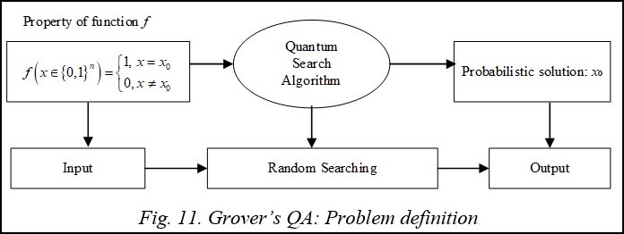
This rule can be understood by considering vectors |iñ and | jñ as column vectors. These vectors belong to the canonical basis, where UF defines a permutation map of the identity matrix rows. In general, row | jñ is mapped into row |iñ.

Quantum block

The heart of the quantum block is the quantum gate, which depends on the properties of matrix UF. The quantum block uses the QAG, which depends on the properties of matrix UF. The structure of a quantum operator UF in QA’s as shown in Fig. 3 is outlined, with a high-level representation, in the scheme diagram of Fig. 8.

The scheme in Fig. 8 gives a more detailed description of the quantum block. The matrix operator UF of Fig. 9 is the output of the encoder block represented in Fig. 3.

Here, it becomes the input for the quantum block. This matrix operator is embedded into a more complex gate: the gate G (QAG). Unitary matrix G is applied k times to an initial canonical basis vector |iñ of dimension 2n+m. Each time, the resulting complex superposition G |0…01…1ñ of basis vectors is measured in measurement block, producing one basis vector |xiñ as result. The measured basis vectors {x1, …, xk} are collected together in block of basis vectors.

This collection is the output of the quantum block. The “intelligence” of the QA’s is in the ability to build a QAG that is able to extract the information necessary to find the required property of f and to store it into the output vector collection.

In order to represent QAG’s it is useful to employ some diagrams called quantum circuits, as shown in Fig. 4. Each rectangle is associated with a matrix 2n ´ 2n, where n is the number of lines entering and leaving the rectangle. For example, the rectangle marked UF is associated with the matrix UF.

Using a high-level description of the gate and, using transformation rules shown in Fig. 10, it is possible to compile the corresponding gate-matrix.

Decoder

The decoder block of Fig. 3 interprets the basis vectors (collected in block basis vectors) of after the iterated execution in the quantum block. Decoding these vectors involves retranslating them into binary strings and interpreting them directly in decoder block if they already contain the answer or use them, for instance as coefficients vectors for some equation system, in order to get the searched solution.

Grover's Problem statement

Grover’s quantum searching problem is stated as following:

Input: Given a function f :{0,1}n®{0,1} such that

.

Problem: Find x.

Figure 11 shows the definition of the Grover's problem.

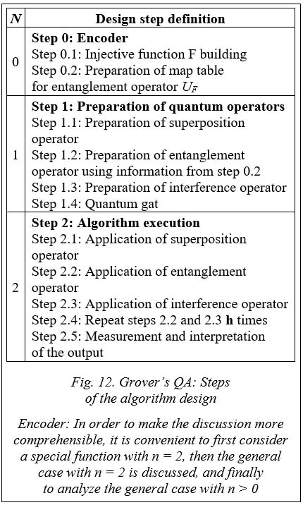
Figure 12 shows step design definitions in Grover's QA.

Design process of Grover’s QAG

Let us consider the implementation of Grover QSA steps in QAG design.

A. Introductory example Consider the case:  n = 2, f(01) = 1. In this case the f map table (see Fig. 9) is defined by:

Step 1

Function f is encoded into injective function F, built according to the usual statement:

Then the F map table is:

Step 2

Now encode F into the map table of UF using the usual rule:

where t is the code map defined in above. This means:

Step 3

From the map table of UF calculate the corresponding matrix operator. This matrix is obtained using the rule: .

UF is thus:

The effect of this matrix is to leave unchanged the first and the second input basis vectors of the input tensor product, flipping the third one when the first vector is |0> and the second is |1>. This agrees with the constraints on UF stated above.

B. General case with n = 2. Now take into consideration the more general case: n = 2, .

The corresponding matrix operator is:

with  

C. General case It is relatively simple now to generalize operator UF from the case n = 2 to the  case n > 1. The operator C is found on the main diagonal of the block matrix, in correspondence of the celled labeled by vector |x>, where x is the binary string having image one by f. Therefore:

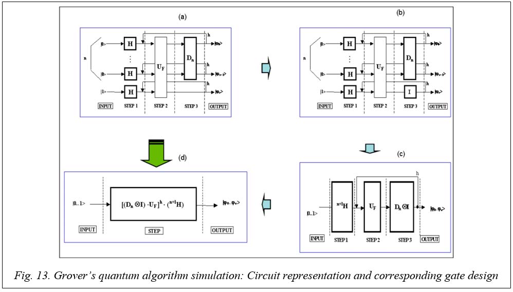
with

Quantum block

The matrix UF, the output of the encoder, is embedded into the QAG.

This gate is described in Fig. 13a, using a quantum circuit of Grover QSA.

Operator Dn is called a “diffusion matrix” of order n and it is responsible for interference in this algorithm. It plays the same role as the QFTn in Shor’s algorithm and of nH in Deutsch–Jozsa’s and Simon’s algorithms. This matrix is defined as:

Using Rule 3 from Fig. 10, compile the previous circuit into the circuit presented as in the Fig. 13, b, and then into the circuit of Fig. 13c and using Rule 2 in Fig. 10 design on Fig. 13d.

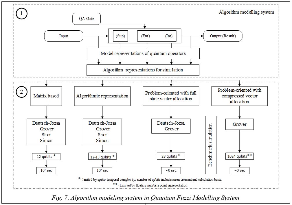
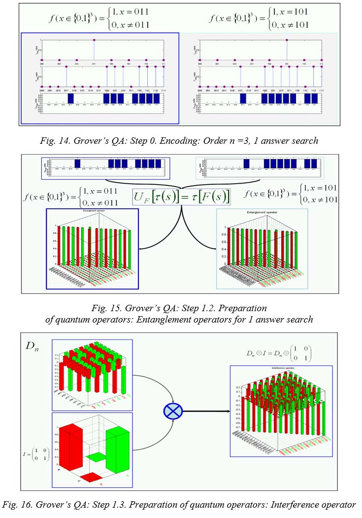
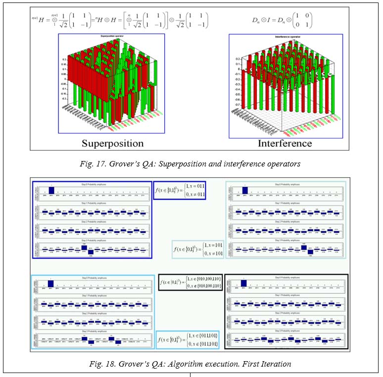
Computer design process of Grover’s QAG and simulation results

Consider the design process of Grover’s QAG according to the steps represented in Fig. 12.

Figure 14 shows Step 0, the encoding process, for the case of order n = 3 and answer search 1.

Preparation of quantum entanglement (step 1.2 from Fig. 12) for the one answer search is shown in Fig. 15.

The cases for 2 and 3 answer searches if the preparation of the entanglement operator is shown by the link http://www.swsys.ru/uploaded/image/ 2023-4/17.jpg.

Figure 16 shows the result of interference operator design (step 1.3 of Fig. 12).

Comparison between superposition and interference operators in Grover’s QAG is shown in Fig. 17.

The Grover’s QAG assembly (step 1.4 of Fig. 12) is shown by the link http://www.swsys.ru/uploaded/ image/2023-4/18.jpg.

The assembled entanglement and interference operators in gate representation (step 1.4 from  Fig. 12) are presented by the link http://www. swsys.ru/uploaded/image/2023-4/19.jpg.

Dynamic evolution of successful results of algorithm execution for the first iteration of Grover’s QAG for initial qubits state |0001ñ and different answer search is shown in Fig. 18.

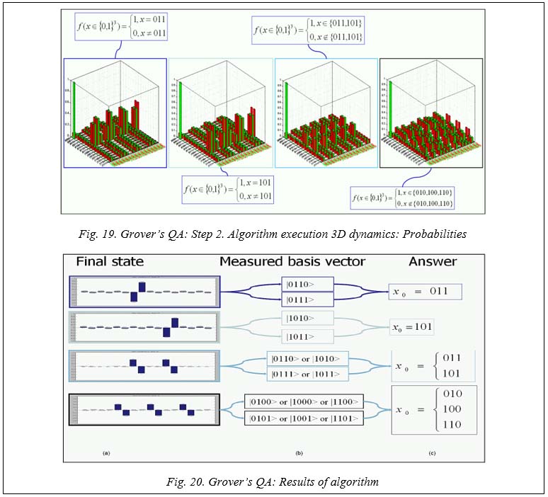
 The algorithm execution results for Grover’s QSA with different number of iterations for successful results with different searching answer number are presented by the link http://www. swsys.ru/uploaded/image/2023-4/20.jpg.

The results of the execution of the RSA Engraver algorithm with a different number of iterations for successful results with different searching answer number

Figure 19 is a 3D dynamic representation  of Grover’s QAG probabilities evolution (step 2 of Fig. 12) for different cases of answer search.

Interpretation of measurement results  in simulation of Grover’s QSA-QAG

In the case of Grover’s QSA this task is achieved (according to the results of this section) by preparing the ancillary qubit of the oracle of the transformation:

in the state . In this case the ope- rator  is computationally equivalent to

and the operator Uf is constructed from a controlled  and two one qubit Hadamard transformations.

Let's show the interpretation of the Grover QAG results.

If measured basis vector: .

Consist of:

.

Then searched argument was:

.

Measured basis vector are computed from the tensor product between the computation qubit re- sults and ancillary measurement qubit. In Grover’s searching process, the ancillary qubit does not change during the quantum computing.

As described above, operator Uf  is constructed from two Hadamard transformations and the Hadamard transformation H (modeling the constructive interference) applied on the state of the standard computational basis can be seen as implementing a fair coin tossing. Thus, if the matrix

 is applied to the states of the standard basis, then H2|0ñ = –|1ñ, H2|1ñ = |0ñ, and therefore H2 acts in measurement process of computational result as a NOT-operation, up to the phase sign. In this case, the measurement basis separated with the computational basis (according to tensor product).

The results of simulation are shown in Fig. 20a. Figure 20b shows the results of computation on a classical computer.

Figure 20b shows two possibilities:

and

.

A similar situation is shown in Fig. 20b.

Figure 20b demonstrate also two searching marked states:

and

A similar situation is shown for three searching marked states in Fig. 20b.

Using a random measurement strategy based on a fair coin tossing in the measurement basis {|0ñ, |1ñ} one can independently receive with certainty the searched marked states from the measurement basis result. Figure 20c show accurate results of searching of corresponding marked states. Final results of interpretation for Grover’s algorithm are shown in Fig. 19. The measurement results based on a fair coin tossing measurement are shown in Fig. 20c.

Figure 20c shows that for both possibilities in implementing a fair coin tossing type of measurement process the search for the answer are successful and demonstrate the possibility of the effective- ness of quantum algorithm simulator realization on classical computer.

Related problems of QA classical simulation  in [6–12] discussed.

Conclusions

General approach to design of quantum algorithm gates is described. Gate-based quantum algorithm representation for effective simulation on computer with classical architecture demonstrated. Grover’s quantum search algorithm is explained in detail along with implementations on a local computer simulator.

References

1.      Grover, L.K. (2001) A Fast Quantum Mechanical Algorithm for Database Search, USA, Pat. US 6,317,766-B1.

2.      Nielsen, M.A., Chuang, I.L. (2000) Quantum Computation and Quantum Information. UK: Cambridge University Press, 676 p.

3.      Serrano, M.A., Perez-Castillo, R., Piattini, M. (2022) Quantum Software Engineering. Springer Verlag Publ., 330 p. doi: 10.1007/978-3-031-05324-5.

4.      Ivancova, O.V., Korenkov, V.V., Ulyanov, S.V., Zrelov, P.V. (2022) Quantum Software Engineering Toolkit. Pt. 1. Moscow, 464 p.

5.      Ulyanov, S.V. (2003) System and Method for Control Using Quantum Soft Computing, USA, Pat. US-6578018-B1.

6.      Nyman, P. (2022) ‘Simulation of quantum algorithms with a symbolic programming language’, ArXiv, art. 0705.3333v2, available at: https://arxiv.org/abs/0705.3333v2 (accessed May 24, 2023).

7.      Juliá-Díaz, B., Burdis, J.M., Tabakin, F. (2009) ‘QDENSITY - A Mathematica quantum computer simulation’, Comput. Phys. Communications, 180(3), pp. 474. doi: 10.1016/j.cpc.2008.10.006.

8.      Johansson, N., Larsson, A.-K. (2017) ‘Efficient classical simulation of the Deutsch–Jozsa and Simon’s algorithms’, Quantum Inf. Process, 16(9), art. 233. doi: 10.1007/s11128-017-1679-7.

9.      Childs, A.M., Coudron, M., Gilani, A.Sh. (2022) ‘Quantum algorithms and the power of forgetting’, ArXiv, art. 2211.12447v2, available at: https://arxiv.org/abs/2211.12447v2 (accessed May 24, 2023).

10.    Cumming, R., Thomas, T. (2022) ‘Using a quantum computer to solve a real-world problem – what can be achieved today?’, ArXiv, art. 2211.13080v1, available at: https://arxiv.org/abs/2211.13080v1 (accessed May 24, 2023).

11.    Abhijith, J., Adedoyin, A., Ambrosiano, J., Anisimov, P. et al. (2022) ‘Quantum algorithm implementations for beginners’, ACM Transactions on Quantum Computing, 3(4), art. 18, pp. 1–92. doi: 10.1145/3517340.

12.    Tezuka, H., Nakaji, K., Satoh, T., Yamamoto, N. (2022) ‘Grover search revisited; application to image pattern matching’, Phys. Rev. A, 105, art. 032440.

Список литературы

1.      Grover L.K. A Fast quantum mechanical algorithm for database search. USA, 2001, Pat. US-6,317,766-B1.

2.      Nielsen M.A., Chuang I.L. Quantum computation and quantum information. UK, Cambridge University Press, 2000, 676 p.

3.      Serrano M.A., Perez-Castillo R., Piattini M. Quantum software engineering. Springer Verlag Publ., 2022, 330 p. doi: 10.1007/978-3-031-05324-5.

4.      Иванцова О.В., Кореньков В.В., Ульянов С.В., Зрелов П.В. Инструментарий квантовой программной инженерии. Ч. 1. М.: Курс, 2022. 464 с. (in Eng.).

5.      Ulyanov S.V. System and method for control using quantum soft computing. USA, 2003, Pat. US-6578018-B1.

6.      Nyman P. Simulation of quantum algorithms with a symbolic programming language. ArXiv, 2022, art. 0705.3333v2. URL: https://arxiv.org/abs/0705.3333v2 (дата обращения: 24.05.2023).

7.      Juliá-Díaz B., Burdis J.M., Tabakin F. QDENSITY – A mathematica quantum computer simulation. Comput. Phys. Communications, 2009, vol. 180, no. 3, pp. 474–474. doi: 10.1016/j.cpc.2008.10.006.

8.      Johansson N., Larsson A.-K. Efficient classical simulation of the Deutsch–Jozsa and Simon’s algorithms. Quantum Inf. Process, 2017, vol. 16, no. 9, art. 233. doi: 10.1007/s11128-017-1679-7.

9.      Childs A.M., Coudron M., Gilani A.Sh. Quantum algorithms and the power of forgetting. ArXiv, 2022, art. 2211.12447v2. URL: https://arxiv.org/abs/2211.12447v2 (дата обращения: 24.05.2023).

10.    Cumming R., Thomas T. Using a quantum computer to solve a real-world problem – what can be achieved today? ArXiv, 2022, art. 2211.13080v1. URL: https://arxiv.org/abs/2211.13080v1 (дата обращения: 24.05.2023).

11.    Abhijith J., Adedoyin A., Ambrosiano J., Anisimov P. et al. Quantum algorithm implementations for beginners. ACM Transactions on Quantum Computing, 2022, vol. 3, no. 4, art. 18, pp. 1–92. doi: 10.1145/3517340.

12.    Tezuka H., Nakaji K., Satoh T., Yamamoto N. Grover search revisited; application to image pattern matching. Phys. Rev. A, 2022, vol. 105, art. 032440.