Авторитетность издания
Добавить в закладки
Следующий номер на сайте


Fast quantum search algorithm modelling on conventional computers: Information analysis of the halting problem
Abstract:The paper describes the simplest technique for simulating a quantum algorithm based on the direct matrix representation of quantum operators. This approach is stable and precise, but it requires allocation of operator’s matrices in the computer memory. Since the size of the operators grows exponentially, this approach is useful for simulating quantum algorithms with a relatively small number of qubits (e.g., approximately 11 qubits on a typical desktop computer). This approach enables relatively simple simulation of the operation of the solution quality control system and performance of a reliability analysis. A more efficient fast quality control simulation method is based on computing all or a part of operator matrices as needed on a current computational basis. This method makes it possible to avoid storing all or a part of the operator matrices. In this case, the number of qubits to be simulated (e.g., the number of input qubits or the number of qubits in the system state register) is affected by: (I) the exponential growth in the number of operations required to calculate the result of matrix products; and (II) the size of the state vector allocated in computer memory. It is reasonable if one embodiment of this approach involves simulating up to 19 or more qubits on typical desktop computer, and even more in a system with a vector architecture. Due to particularities of the memory addressing and access processes in a typical desktop computer (such as, for example, a Pentium PC), when a number of qubits is relatively small, the on-demand computing tends to be faster than the direct storage approach. The compute-on-demand approach benefits from applying the results of studying quantum operators and their structure that enables computing the matrix elements more efficiently. The paper considers effective simulation of Grover’s quantum search algorithm using a computer with classical architecture.
Аннотация:Описана методика модификации моделирования квантового алгоритма, основанная на прямом (большого объема) матричном представлении квантовых операторов. Этот подход стабилен и точен, но требует размещения матриц оператора в памяти компьютера. Поскольку размер операторов растет экспоненциально, подход полезен для моделирования квантовых алгоритмов с относительно небольшим количеством кубитов (например, приблизительно 11 кубитов на типовом компьютере). Используя его, относительно просто смоделировать работу системы контроля качества решения и выполнить анализ достоверности. Более эффективный метод быстрого моделирования контроля качества основан на вычислении всех или части операторных матриц по мере необходимости на текущей вычислительной основе. Используя данный метод, можно избежать сохранения всех или части операторных матриц. В этом случае количество кубитов, которые могут быть смоделированы (например, количество входных кубитов или количество кубитов в регистре состояния системы), влияет на экспоненциальный рост числа операций, необходимых для вычисления результата матричных произведений, и на размер вектора состояния, выделяемого в памяти компьютера. В одном из вариантов применения этого подхода целесообразно моделировать до 19 или более кубитов на типичном настольном компьютере и даже больше на системе с векторной архитектурой. Из-за особенностей процессов адресации памяти и доступа к ней в типичном настольном компьютере (например, персональный компьютер на базе Pentium), когда количество кубитов относительно невелико, подход «вычисления по требованию», как правило, эффективнее, чем подход с прямым хранением. Подход «вычисления по требованию» выигрывает благодаря применению результатов детального изучения квантовых операторов и их структуры, что позволяет более эффективно вычислять матричные элементы. В работе рассмотрено эффективное моделирование алгоритма квантового поиска Гровера на примере компьютера с классической архитектурой.
| Авторы: Ульянов С.В. (ulyanovsv46_46@mail.ru) - Государственный университет «Дубна» – Институт системного анализа и управления, Объединенный институт ядерных исследований – лаборатория информационных технологий (профессор), Дубна, Россия, Ph.D, Ульянов В.С. (ulyanovik@mail.ru) - Московский государственный университет геодезии и картографии (МИИГАиК) (доцент), Москва, Россия, Ph.D | |
| Keywords: termination criteria, minimum of Shannon information entropy, quantum computing, algorithmic representation, state vector, quantum operators, fast quantum search algorithm |
|
| Ключевые слова: критерии завершения, минимум информационной энтропии шеннона, квантовые вычисления, алгоритмическое представление, вектор состояния, квантовые операторы, алгоритм быстрого квантового поиска |
|
| Количество просмотров: 1406 |
Статья в формате PDF |
The study of the on-demand computing approach for some quantum algorithms (QAs) can lead to a problem-oriented approach based on the quantum algorithm (QA) structure and state vector behavior [1–3]. For example, in Grover’s quantum search algorithm (QSA) [4], the state vector always has one of the two different values: (I) one value corresponds to the probability amplitude of the answer; and (II) the second value corresponds to the probability amplitude of the rest of the state vector. Based on this assumption, it is possible to configure the algorithm using these two different values, and to efficiently simulate Grover’s QSA. In this case, the primary limit is a representation of the floating-point numbers used to simulate the actual values of the probability amplitudes. After the superposition operation, these probability amplitudes are very small
Other QAs do not necessarily reduce to just two values. For those algorithms that reduce to a finite number of values, we can use the techniques for simplifying the Grover’s QSA, but the maximum number of input qubits to be simulated will tend to be smaller, because the probability amplitudes of other algorithms have relatively more complicated distributions. Introduction of an external excitation can decrease the possible number of qubits for some algorithms. In some algorithms, the entanglement and interference operators can be bypassed (or simplified), and the output is computed based only on a superposition of the initial states (and deconstructive interference of the final output patterns) representing the state of the designed schedule of control gains. For example, it is possible to make a particular case of Deutsch-Jozsa’s and Simon algorithms entanglement-free by using pseudo-pure quantum states [5]. The further disclosure begins with a comparative analysis of the temporal complexity of several representative QAs. The analysis is followed by an introduction of the generalized approach in QA simulation and algorithmic representation of quantum operators. Subsequent portions describe the structure representation of the QAs applicable to low level programming on classical computer (PC), generalizations of the approaches and intro- duction of the general QA simulation tool based on fast problem-oriented QAs. The simulation techniques are then applied to a quantum control algorithm. It is possible to efficiently implement the matrix-based approach for a small number of input qubits. The above-mentioned matrix approach is a useful tool to illustrate complexity issues associated with QA simulation on classical computer. The structure of the QA gate system design As shown in Fig. 1a, QA simulation can be represented as a generalized representation of a QA as a set of sequentially applied smaller quantum gates (see in details [1]). Moreover, local optimization of QA components according to specific hardware realization makes it possible to develop appropriate hardware accelerators for QA simulation using classical gates. A generalized approach in QA simulation
Layer 1: Input. The quantum state vector is set up to an initial value for this certain algorithm. For example, the input for Grover’s QSA is a quantum state |f0ñ described as a tensor product:
where
The coefficients ai in Eq. (1) are called probability amplitudes. Probability amplitudes can take negative and/or complex values. However, the probability amplitudes must obey the following constraint:
The actual probability of the arbitrary quantum state Layer 2: Superposition. The Walsh-Hadamard operator transforms the state of the quantum state vector so that probabilities are distributed uniformly among all basis states. The result of the superposition layer of Grover’s QSA is shown in Fig. 2b as a probability amplitude representation, and in Fig. 3b as a probability representation. Layer 3: Entanglement. Probability amplitudes of the basis vector corresponding to the current problem are flipped while rest basis vectors are left unchanged. Entanglement is typically provided by controlled-NOT (CNOT) operations. Figs 2c and 3c show the results of entanglement from the application of the operator to the state vector after superposition operation. An entanglement operation does not affect the probability of the state vector to be measured. Rather, entanglement prepares a state, which cannot be represented as a tensor product of simpler state vectors. For example, let us consider state f1 shown in Fig. 2b and state f2 presented in Fig. 2c:
As shown above, the description of state f1 can be presented as a tensor product of simpler states, while state f2 (in the measurement basis Layer 4: Interference. Probability amplitudes are inverted about the average value. As a result, the probability amplitude of states ²marked² by entanglement operation will increase. Figs 2d and 3d show the results of interference operator application. Fig. 2d shows probability amplitudes and Fig. 3d shows probabilities. Layer 5: Output. The output layer provides the measurement operation (extraction of the state with maximum probability) followed by interpretation of the result. For example, in the case of Grover’s QSA, the required index is coded in the first Since unitary quantum operators implement various QA layers, simulation of quantum operators depends on simulating such unitary operators. Thus, in order to develop an efficient simulation, it is useful to understand the nature of QA basic quantum operators. Basic QA operators Let us consider the superposition, entanglement and interference operators from the simulation point of view. In this case, the superposition operators and the interference operators have more complicated structure and differ from algorithm to algorithm. Thus, it is first useful to consider the entanglement operators, since they have a similar structure for all QAs, and differ only by the analyzed function. In general, the superposition operator is based on the combination of the tensor products Hadamard H operators: Remark. As described in [1–3] the simulation system of quantum computation is based on quantum algorithm gates (QAG). The design process of QAG includes the matrix design form of three quantum operators: superposition (Sp), entanglement (UF) and interference (Int). In a general form, we can describe the structure of a QAG as follows:
where I is the identity operator; the symbol Ä denotes a tensor product; S is equal to I or H and depends on the problem description. One portion of the design process in QAG is the type-choice of the entanglement problem-dependent operator UF that physically describes the qualitative properties of the function f. The Hadamard Transform creates the superposition on classical states, and quantum operators such as CNOT create robust entangled states. The Quantum Fast Fourier Transform (QFFT) pro- duces interference. For most QAs the superposition operator can be expressed as
where n and m are the numbers of inputs and of outputs respectively. The operator S depends on the algorithm and can be either the Hadamard operator H or the identity operator I. The numbers of outputs m as well as structures of the corresponding superposition and interference operators are presented in Table 1 for different QAs. Table 1 Parameters of superposition and interference operators of main quantum algorithms
Superposition and interference operators are often constructed as tensor powers of the Hadamard operator, which is called the Walsh-Hadamard operator. Elements of the Walsh-Hadamard operator can be obtained as
where i = 0,1, j = 0,1, H denotes Hadamard matrix of order 3. The rule in Eq. (4) provides a way to speed up the classical simulation of the Walsh-Hadamard operators, since the elements of the operator can be obtained by a simple replication described in Eq. (4) from the elements of the n–1H order operator. As an example, we consider the superposition operator of Grover’s algorithm, for n = 2, m = 1, S = H:
Interference operators are calculated for each algorithm according to the parameters listed in Table 1. The interference operator is based on the interference layer of the algorithm, which is different for various algorithms, and from the measurement layer, which is the same or similar for most algorithms and includes mth tensor power of the identity operator. The interference operator of the Grover’s algorithm can be written as a block matrix in the following form:
where For example, the interference operator for Grover’s QSA when n = 2, m = 1 is:
As the number of qubits increases, the gain coefficient becomes smaller. The dimension of the matrix increases according to 2n, but each element can be extracted using Eq. (6), without allocation of the entire operator matrix. Remark. Since In a specific form the operator Dn (diffusion – inversion about average) in Grover algorithm is decomposed as
and can be accomplished with O(n) = O(log(n)) quantum gates. It means that from the viewpoint of efficient computation the form in Eq. (6) is more preferable. An entanglement operator is a sparse matrix. Using sparse matrix operations, it is possible to accelerate the simulation of the entanglement. Each row or column of an entanglement operation has only one position with a non-zero value. This is a result of the function F reversibility. For example, let us consider the entanglement operator for a binary function with two inputs and one output:
The reversible function F in this case is:
The corresponding entanglement block matrix can be written as:
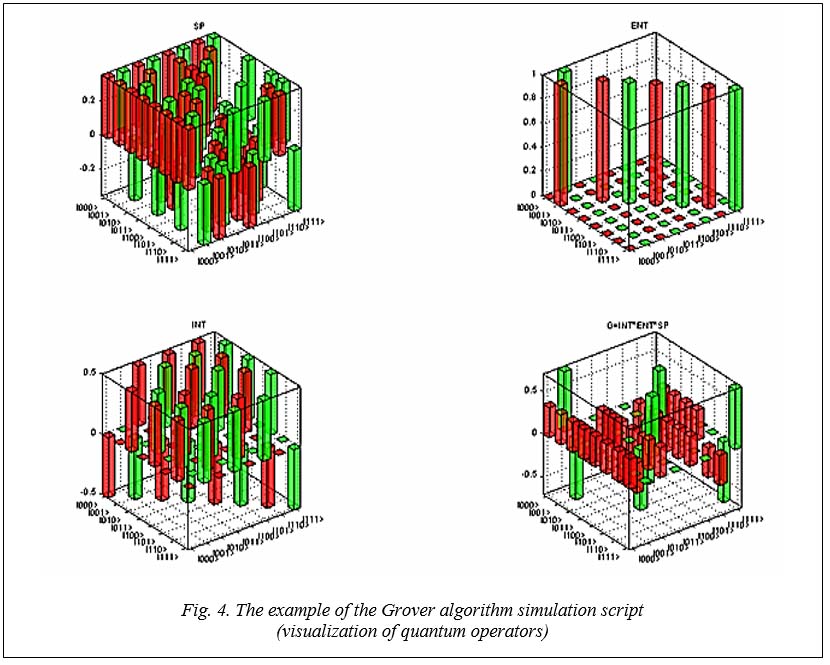
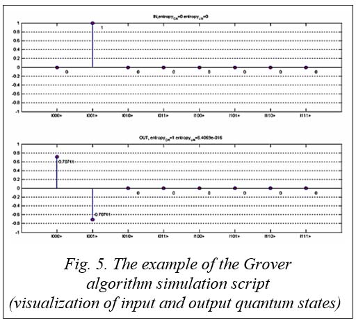
Figure 2c shows the result applying this operator in Grover’s QSA. Command line simulation of the QAs Let us present an example script of the Grover's algorithm (http://www.swsys.ru/uploaded/image/ 2023-3/2023-3-dop/17.jpg, http://www.swsys.ru/uploaded/image/2023-3/2023-3-dop/18.jpg, http:// www.swsys.ru/uploaded/image/2023-3/2023-3-dop/19.jpg). The algorithm-related script (http://www. swsys.ru/uploaded/image/2023-3/2023-3-dop/ 17.jpg) prepares the superposition (SP), entanglement (ENT) and interference (INT) operators of the Grover’s algorithm with 3 qubits (including the measurement qubit). Then it assembles operators into the quantum gate G. Then this script creates an input state |in > = |001> and calculates the output state |out > = G| in >. The result of this algorithm in Matlab is an allocation of operator matrices and state vectors in the memory.
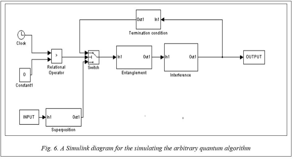
In this case, the vertical axis corresponds to the amplitudes of the corresponding matrix elements. Indexes of the elements are marked with the ket notation. Input |in> and the output |out> states are demonstrated in Fig. 5. In this case, the vertical axis corresponds to the probability amplitudes of the state vector components. The horizontal axis corresponds to the index of the state vector component marked by the ket notation. The title of the Fig. 5 contains the values of the Shannon and the von Neumann entropies of the corresponding visualized states. We can formulate and execute other known QA using similar scripts and the corresponding equations taken from the previous section. Simulating QAs as dynamic systems In order to simulate the behavior of dynamic systems with quantum effects, it is possible to represent QA as a dynamic system in the form of a block diagram and then to simulate its behavior in time. The example of a Simulink diagram of the quantum circuit for calculating the accuracy The ket function output goes to the first input of the matrix multiplier and as a second input of the matrix multiplier. The input also proceeds to the bra function. The output of the bra function goes to the second input of the matrix multiplier and as the first input of the matrix multiplier. The multiplier output is a density matrix of the input state. The multiplier output is the input state fidelity.
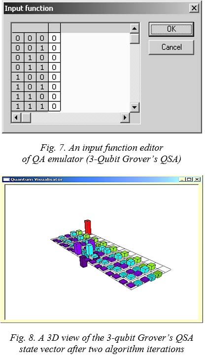
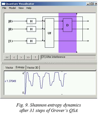
Such structure can be used to simulate a number of quantum algorithms in Matlab/Simulink environment. A dedicated QA emulator The developed QA algorithmic representation is also applicable for designing QA software emulators. The key point is the reduction of multiple matrix operations to vector operations and the following replacement of multiplication operations. This may boost emulation performance, especially in the algorithms which do not require complex number operations, and when a quantum state vector has a relatively simple structure (for example, Grover’s QSA). In the QC emulator launch window (http:// www.swsys.ru/uploaded/image/2023-3/2023-3- dop/21.jpg), we can choose creating a new QC model or continue modeling an existing one. If we choose creating a new model, then an algorithm selection dialog starts (http://www.swsys.ru/ uploaded/image/2023-3/2023-3-dop/22.jpg). Here a user may choose QA and its dimensions. In fact, the system may operate with up to 50 qubits and more, however due to visualization problems, it is better to limit number of qubits to 10–11. Once the algorithm initial parameters are set, the system draws an initial state vector and the selected algorithm structure in the system main window (http://www.swsys.ru/uploaded/image/2023-3/2023-3-dop/23.jpg). The main window contains all information of the emulated quantum algorithm and permits basic operations and analysis. There is an access to involved quantum operators from the menu, and it is possible to modify input functions (http://www. swsys.ru/uploaded/image/2023-3/2023-3-dop/24.jpg, http://www.swsys.ru/uploaded/image/ 2023-3/2023-3-dop/25.jpg). QAs have reversible nature, so it is possible to make forward and backward steps of the algorithm by clicking on arrows, and the currently applied algorithm step will be highlighted in the algorithm diagram. The emulator menu consists of four components: 1. Item File provides basic operations like project save/load and an access to the new model creation interface. 2. Item Model permits an access to the input function editor. 3. Item View provides an access to operator matrix visualizers including Superposition, Entanglement and Interference operators. It is also possible to get a 3D preview of an algorithm state dynamics (Fig. 4). 4. There is an access to the program documentation from Help menu. Tabbed interface in the lower part of the window gives an access to the Shannon entropy chart and to a 3D representation of the state vector dynamics, as well as to a usual, plain representation of the QA state. The tabbed area size can be modified by dragging a divider. A click on the middle point of divider hides the tabbed area form the screen. The buttons in the middle part of the main window permit making steps of the currently parameterized QA. As it was mentioned above, the system can make forward and backward steps. If the algorithm steps were enough, a click on the ²!² button will extract an answer from the current state vector. An appropriate result interpretation routine will be called depending on QA. The quantum operator visualizer permits displaying a structure of involved quantum operator matrices in plain and in 3D representations. If an operator consists of a tensor product of smaller operators, there is also a possibility to have an access to sub-blocks of the tensor products. A 3D visualizer permits zoom and rotation of the charts. The input function editor enables automating the process of the entanglement operator coding as it was described previously. For Grover’s QSA it is possible to code functions with more than one positive output (Fig. 7).
The developed software can simulate 4 basic quantum algorithms, e.g. Deutsch-Jozsa’s, Shor’s, Simon’s and Grover’s. The system uses a unified easy-to-understand interface for all algorithms, with the options of 3D visualization of state vector dynamics and quantum operators. After analyzing quantum operators presented in the section 5, we can do the following simplification to increase the performance of classical QA simulations: a) all quantum operators are symmet- rical around main diagonal matrices; b) a state vector is allocated as a sparse matrix; c) elements of quantum operators are not stored, but calculated when necessary using Eqs. (4), (5), (6) and (7); d) we consider minimum of Shannon entropy of the quantum state as a termination condition, calculated as:
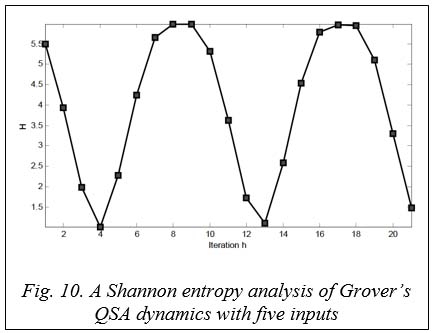
The calculation of the Shannon entropy is applied to a quantum state after the interference operation [6, 7]. The results of a classical quantum algorithmic gate simulation Minimum of the Shannon entropy Eq. (8) corresponds to the state when there are few state vectors with high probability (states with minimum uncertainty). Selecting an appropriate termination condition is important since QAs are periodical. Figure 10 shows results of the Shannon information entropy calculation for Grover’s algorithm with 5 inputs.
Simulation results of fast Grover QSA are summarized in Table 2. Table 2 Temporal complexity of Grover’s QSA simulation on 1.2GHz computer with two CPUs
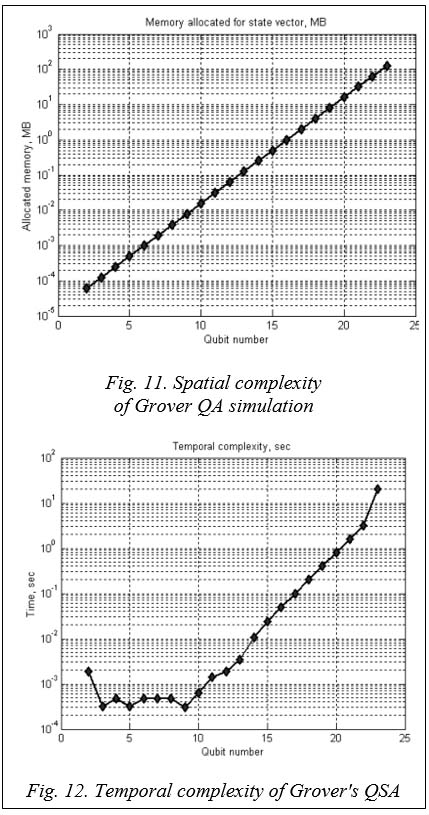
Numbers of iterations for fast algorithm were estimated according to termination condition as the minimum of the Shannon entropy of a quantum state vector. The simulation involved the following approaches: Approach 1: Quantum operators are applied as matrices; elements of quantum operator matrices are calculated dynamically according to Eqs. (5), (6), and (7). Classical Hardware limit of this approach is around 20 qubits caused by exponential temporal complexity. Approach 2: Quantum operators are replaced with classical gates. Product operations are removed from simulation according to [8]. A state vector of probability amplitudes is stored in a compressed form (only different probability amplitudes are allocated in memory). The second approach makes it possible to perform classical efficient simulation of Grover’s QSA with an arbitrary large number of inputs (50 qubits and more). When allocating the state vector in computer memory, this approach permits simulating 26 qubits on PC with 1GB of RAM. Figure 11 shows memory required for Grover algorithm simulation, when the whole state vector is allocated in memory. Adding one qubit requires doubling the computer memory needed for simulating Grover's QSA in case when a state vector is allocated completely in memory.
In this case, the state vector is allocated in memory and quantum operators are replaced with classical gates according to [8]. The fastest case is when we compress the state vector and replace quantum operator matrices with corresponding classical gates according to [8]. In this case, we obtain speedup according to Approach 2. Fast QSA models: The structure and acceleration method of quantum algorithm simulation The analysis of the quantum operator matrices carried out in the previous sections forms the basis for specifying structural patterns that give the background for the algorithmic approach to QA modeling on classical computers. Allocating only a fixed set of tabulated (pre-defined) constant values in the computer memory instead of allocating huge matrices (even in sparse form) provides computational efficiency. Various elements of the quantum operator matrix can be obtained by applying an appropriate algorithm based on structural patterns and particular properties of the equations that define matrix elements. Each representation algorithm uses a set of table values for calculating matrix elements. Calculation of the tables of the predefined values can be done as a part of the algorithm initialization.
Here n is a number of qubits, i and j are the indexes of a requested element, In Fig. 13a, the i, j values are specified and provided to an initialization block with loops control variables ii := i, jj := 0, and k := 0 are initialized, and a calculation variable h := 1 is initialized. Then the process moves to a decision block. In the decision block, if k is less than or equal to n, then the process advances to another decision block; other- wise, the process advances to an output block where the output h*hc is computed (where In the decision block, if (ii and jj and 1) = 1, then the process advances to a block h := –h; otherwise, the process advances to another block and passes to the next iteration without probability amplitude inversion. Alternatively, the process sets h := –h and proceeds to the next iteration. By setting ii := ii SHR 1, jj := jj SHR 1, and k := k + 1 (where SHR is a shift right operation), and then the process continues until all probability amplitudes are assigned. In Fig. 13, the inputs i, j in an input block are initialized as ii := i SHR 1, and jj := SHR 1 and then are passed to the end test. If the end test fail, it means that the inputs i and j are pointing to the marked elements; in this case the process of the probability amplitude inversion of the marked states is performed. In Fig. 13c, the interference operator of Grover’s QSA can be substituted by a simple logic algorithm that outputs 0 if ((i XOR j) AND 1) = 1. Then regarding nonzero elements, if i = j then dc1 outputs the process, otherwise dc2, where The superposition and entanglement operators for Deutsch-Jozsa’s QA are the same as superposition and entanglement operators for Grover’s QSA (Figs 13a,b), respectively). The time required for calculating the elements of an operator’s matrix during a process of applying a quantum operator is generally small in comparison to the total time of performing a quantum step. Thus, the live load created by exponentially increasing memory usage tends to be less or at least similar to the live load created by computing matrix elements as needed. Moreover, since the algorithms for computing matrix elements tend to be based on fast bit-wise logic operations, algorithms are amenable to hardware acceleration. Table 3 shows comparisons of the traditional and required matrix calculation when the memory is used for the algorithm as required (Memory* is memory used for storing the quantum system state vector). Table 3 shows that the algorithmic approach enables a significant speed-up compared with the prior art direct matrix approach. The use of algorithms for providing matrix elements allows considerable software optimization, including the ability to optimize at the machine instruction level. However, as the number of qubits increases, there is an exponential increase in temporal complexity, which shows itself as an increase in time required for matrix product calculations. Table 3 Different approaches comparison: Standard (matrix based) and algorithmic-based approach
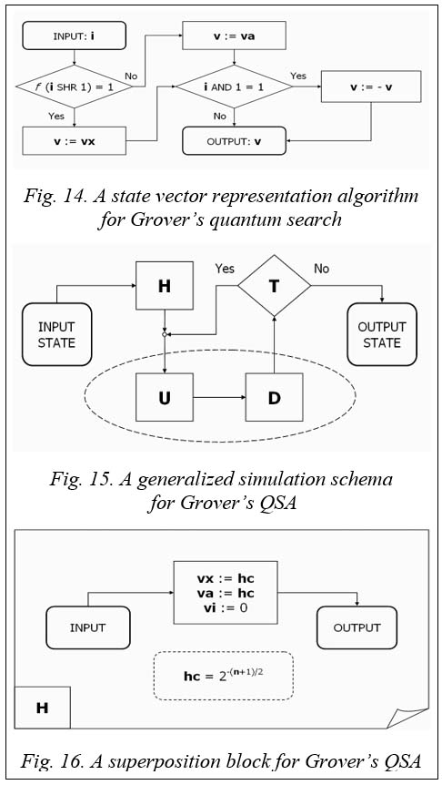
* The results shown in Table 3 are based on the results of testing the software implementation of the Grover QSA simulator on a personal computer with Intel Pentium III 1 GHz processor and 512 Mb memory. Only one iteration of the Grover QSA was performed. Using structural patterns in the quantum system state vector and a problem-oriented approach for each particular algorithm can compensate this increase in temporal complexity. By way of explanation and not by way of limitation, the Grover algorithm is used below to explain the problem-oriented approach to simulating QA on a classical computer. The problem-oriented approach based on a structural pattern of QA state vector Let n be the input number of qubits. In the Grover algorithm, half of all Odd 2n elements can be classified into two categories: - A set of m elements corresponding to truth points of an input function (or oracle); - The remaining 2n – m elements. The values of the same category elements are always equal. As discussed above, Grover’s QA only requires two variables for storing element values. Its limitation in this sense depends only on a computer representation of the floating-point numbers used for state vector probability amplitudes. For a double-precision software implementation of the state vector representation algorithm, the upper reachable limit of q-bit number is approximately 1024. Figure 14 shows a state vector representation algorithm for Grover’s QA. In Fig. 14 Classical gates are used not for simulating appropriate quantum operators with strict one-to-one correspondence but for simulating a quantum step that changes the system state. Matrix product operations are replaced by arithmetic operations with a fixed number of parameters irrespective of a qubit number. Figure 15 shows a generalized schema for efficient simulation of the Grover QA built upon three blocks, a superposition block H, a quantum step block UD and a termination block T.
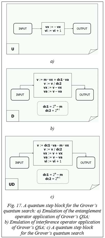
As shown in Fig. 16, the superposition block H for Grover’s QSA simulation changes the system state to the state obtained traditionally by using n + 1 times the tensor product of Walsh-Hadamard transformations. In the process shown in Fig. 13, vx := hc, va := hc, and vi := 0, where The quantum step block UD that emulates the entanglement and interference operators is shown on Figs 17a–c. The UD block reduces the temporal complexity of the quantum algorithm simulation to a linear dependence on the number of executed iterations. The UD block uses recalculated table values In the U block shown in Fig. 17, vx := – vx and vi := vi + 1. In the D block shown in Fig. 17b, v := m*vx+dc1*va, v := v/dc2, vx := v – vx, and va := v – va; in the UD block shown in Fig. 17c, v := dc1*va = m*vx, v := v/dc2, vx := v + vx, va := := v – va, and vi := vi + 1. The termination block T is general for all QAs without regard to the operator matrix realization. Block T provides intelligent termination condition for a search process. Thus, the block T controls the number of iterations through the block UD by providing enough iteration to achieve a high probability of arriving at a correct answer to the search problem. The block T uses a rule based on observing the changing of the vector element values according to two classification categories. During a number of iterations, T block check that the values of same category elements monotonically increase or decrease while values of other category elements changed monotonically in reverse direction. If the direction is changed after some number of iterations, it means that an extremum point corresponding to a state with maximum or minimum uncertainty is passed. The process can use direct values of amplitudes instead of considering Shannon entropy value, thus, it significantly reduces the re- quired number of calculations for determining the minimum uncertainty state that guarantees the high probability of a correct answer. The termination algorithm implemented in T block can use one or more of five different termination models: Model 1: Stop after a predefined number of iterations; Model 2: Stop on the first local entropy minimum; Model 3: Stop on the lowest entropy within a predefined number of iterations; Model 4: Stop on a predefined level of acceptable entropy; and/or Model 5: Stop on the acceptable level or lowest reachable entropy within the predefined number of iterations. Note that models 1–3 do not require calculating an entropy value.
Since time efficiency is one of the major demands on such termination condition algorithm, a separate module represents each part of the termination algorithm; and before the termination algorithm starts, links are built between the modules in correspondence to the selected termination model by initializing the appropriate functions’ calls. Table 4 shows components for the termination condition block T for the various models. Table 4 Termination block construction
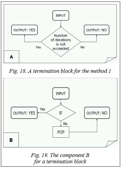
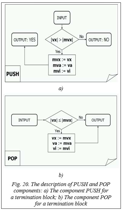
The elements A, B, PUSH, C, D, E, and PUSH-code in Table 4 correspond to the flowcharts (http://www.swsys.ru/uploaded/image/2023-3/ 2023-3-dop/26.jpg, http://www.swsys.ru/uploaded/ image/2023-3/2023-3-dop/27.jpg, http://www. swsys.ru/uploaded/image/2023-3/2023-3-dop/ 28.jpg). In model 1 requires only one test after each application of quantum step block UD, block A performs this test. Therefore, the initialization includes assuming A to be T, i.e., function calls to T are addressed to block A shown in Fig. 18. As shown in Fig. 18, A block checks if the maximum number of iterations has been reached, if so, then the simulation is terminated, otherwise the simulation continues. In model 2, simulation stops when the direction of category value modification is changed. Model 2 uses the comparison of the current value of vx category with mvx value that represents this category value obtained in previous iteration: I. If vx is greater than mvx, its value is stored in mvx, vi value is stored in mvi, and the termination block proceeds to the next quantum step; II. If vx is less than mvx, it means that vx maximum is passed and the process needs to set the current (final) value of vx := mvx, vi := mvi, and stop the iteration process. So, the process stores the maximum of vx in mvx and the appropriate iteration number vi in mvi. Here block B, shown in Fig. 19 is used as the main block of the termination process.
In the POP block in Fig. 17b, if |vx| <= |mvx|, then vx := mvx, va := mva, and vi := mvi. The model 3 termination block checks to see that a predefined number of iterations do not exceed (using block A in Fig. 20): - If the check is successful, then the termination block compares the current value of vx with mvx. If mvx is less than, it sets the value of mvx equal to vx and the value of mvi equal to vi. If mvx is less using the PUSH block, then perform the next quantum step; - If the check operation fails, then (if needed) the final value of vx equal to mvx, vi equal to mvi (using the POP block) and the iterations stop. The model 4, the termination block uses a single component block D (http://www.swsys.ru/up- loaded/image/2023-3/2023-3-dop/27.jpg). The D block compares the current Shannon entropy value with a predefined acceptable level. If the current Shannon entropy is less than the acceptable level, then the iteration process is stopped; otherwise, the iterations continue. The model 5 termination block uses the A block to check that a predefined number of iterations do not exceeded. If the maximum number is exceeded, then the iterations are stopped. Otherwise, the D block is then used to compare the current value of the Shannon entropy with the predefined acceptable level. If an acceptable level is not achieved, then the PUSH block is called and the iterations continue. After the last performed iteration, the POP block is called to restore the vx category maximum and appropriate vi number and the iterations end.
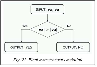
If |vx| > |va|, then the search was successful; otherwise the search was not successful. Table 5 lists the results of testing the optimized version of Grover QSA simulator on a personal computer with Pentium 4 processor at 2GHz. Using the above algorithm, a simulation of a 1000 qubit Grover QSA requires only 96 seconds for 108 iterations (http://www.swsys.ru/up-loaded/ image/2023-3/2023-3-dop/29.jpg). The theoretical boundary of this approach is not the number of qubits, but the representation of the floating-point numbers. Table 5 High probability answers for Grover QSA
The practical bound is limited by the front side bus frequency of a personal computer. Related works. The presented approach was firstly suggested in [9–11] for efficient simulation of quantum algorithms on classical computers with minimum Shannon entropy measure of termination of searching processes [7] and differ from results in [12–16] and [17–20]. Conclusions In this paper we have: presented a design method of a modular system for realization of the Grover’s Quantum Search Algorithm; developed a design process of main quantum operators with algorithmic description for quantum algorithm gates simulation on a classical computer. We also have: introduced model representations of quantum operators in fast QAs; described an algorithmic based approach when matrix elements are calculated on demand; demonstrated a problem-oriented approach, where we succeeded to run Grover’s algorithm with up to 64 and more qubits with Shannon entropy calculation (up to 1024 without termination condition) and considered it as a solution of a classically intractable problem. These results are the background for efficient simulation of quantum soft computing algorithms on a classical computer, robust fuzzy control based on quantum genetic (evolutionary) algorithms and quantum fuzzy neural networks (that can implemented as modified Grover’s QSA), AI-problems as quantum game’s gate simulation approaches and quantum learning, quantum associative memory, quantum optimization. Reference List 1. Nielsen, M.A., Chuang, I.L. (2000) Quantum Computation and Quantum Information. UK: Cambridge University Press, 676 p. 2. Serrano, M.A., Perez-Castillo, R., Piattini, M. (2022) Quantum Software Engineering. Springer Verlag Publ., 330 p. 3. Korenkov, V.V., Reshetnikov, A.G., Ulyanov, S.V. (2022) Quantum Software Engineering. Vol. 2. Moscow, 452 p. 4. Grover, L.K. (2001) A Fast Quantum Mechanical Algorithms, US, Pat. 6,317,766 B1. 5. Ivancova, O.V., Korenkov, V.V., Ulyanov, S.V. (2020) Intelligent Computing Technologies. Pt. 2. Quantum Computing and Algorithms. Quantum Self-Organization Algorithm. Quantum Fuzzy Inference. Moscow: Kurs Publ., 296 p. 6. Ulyanov, S.V., Panfilov, S.A., Kurawaki, I., Yazenin, A.V. (2001) ‘Information analysis of quantum gates for simulation of quantum algorithms on classical computers’, in QCM&C, pр. 207–214. doi: 10.1007/0-306-47114-0_32. 7. Ghisi, F., Ulyanov, S.V. (2000) ‘The information role of entanglement and interference in Shor quantum algorithm gate dynamics’, J. of Modern Optics, 47(12), pp. 2079–2090. doi: 10.1080/09500340008235130. 8. Amato, P., Ulyanov, S., Porto, D., Rizzotto, G.G. (2003) ‘Hardware architecture system design of quantum algorithm gates for efficient simulation on classical computers’, Proc. SCI, 3, pp. 398–403. 9. Panfilov, S.A., Ulyanov, S.V., Litvintseva, L.V., Yazenin, A.V. (2004) ‘Fast algorithm for efficient simulation of quantum algorithm gates on classical computer’, Systemics, Cybernetics and Informatics, 2(3), pp. 63–68. 10. Ulyanov, S.V. (2003) System and Method for Control Using Quantum Soft Computing, US, Pat. 6,578,018 B1. 11. Ulyanov, S.V., Panfilov, S.A. (2006) Efficient Simulation of Quantum Algorithm Gates on Classical Computer Based on Fast Algorithm, US, Pat. 2006/0224.547 A1. 12. Nyman, P. (2007) ‘Simulation of quantum algorithms with a symbolic programming language’, ArXiv, art. 0705.3333v2, available at: https://arxiv.org/abs/0705.3333v2 (accessed November 18, 2022). 13. Juliá-Díaz, B., Burdis, J.M., Tabakin, F. (2009) ‘QDENSITY – A Mathematica quantum computer simulation’, CPC, 180(3), art. 474. doi: 10.1016/j.cpc.2008.10.006. 14. Cumming, R., Thomas, T. (2022) ‘Using a quantum computer to solve a real-world problem – what can be achieved today?’, ArXiv, art. 2211.13080v1, available at: https://arxiv.org/abs/2211.13080v1 (accessed November 18, 2022). 15. Ovide, A., Rodrigo, S., Bandic, M., Van Someren, H., Feld, S. et al. (2023) ‘Mapping quantum algorithms to multi-core quantum computing architectures’, ArXiv, art. 20232303.16125v1, available at: https://arxiv.org/pdf/2303.16125.pdf (accessed November 18, 2022). 16. Abhijith, J., Adedoyin, A., Ambrosiano, J., Anisimov, P. et al. (2022) ‘Quantum algorithm implementations for beginners’, ArXiv, art. 1804.03719v3, available at: https://arxiv.org/abs/1804.03719v3 (accessed June 27, 2022). 17. Tezuka, H., Nakaji, K., Satoh, T., Yamamoto, N. (2021) ‘Grover search revisited; application to image pattern matching’, ArXiv, art. 2108.10854v2, available at: https://arxiv.org/abs/2108.10854v2 (accessed Oct 1, 2021). 18. Vlasic, A., Certo, S, Pham, A. (2022) ‘Complement Grover’s search algorithm: An amplitude suppression implementation’, ArXiv, art. 2209.10484v1, available at: https://arxiv.org/abs/2209.10484 (accessed September 27, 2022). 19. Chattopadhyay, A., Menon, V. (2021) ‘Fast simulation of Grover’s quantum search on classical computer’, ArXiv, art. 2005.04635, available at: https://arxiv.org/pdf/2005.04635.pdf (accessed September 27, 2022). 20. Toffano, Z., Dubois, F. (2020) ‘Adapting logic to physics: The quantum-like eigenlogic program’, Entropy, 22(2), art. 139. doi: 10.3390/e22020139. Список литературы
| |||||||||||||||||||||||||||||||||||||||||||||||||||||||||||||||||||||||||||||||||||||||||||||||||||||||||||||||||||||||||||||||||||||||||||||||||||||||||||||||||||||||||||||||||

 (1)
(1)
 (4)
(4) (5)
(5)
 (7)
(7)


| Постоянный адрес статьи: http://swsys.ru/index.php?page=article&id=5011 |
Версия для печати |
| Статья опубликована в выпуске журнала № 3 за 2023 год. [ на стр. 361-377 ] |
Возможно, Вас заинтересуют следующие статьи схожих тематик:
- Программный эмулятор квантовых алгоритмов для эффективного моделирования на персональном компьютере
- Оптимизация размещения средств траекторных измерений генетическими алгоритмами
- Оценка возможностей классических компьютеров при реализации симуляторов квантовых алгоритмов
- Квантовый генетический алгоритм в задачах моделирования интеллектуального управления и суперкомпьютинг
- Интеллектуальное робастное управление роботом-манипулятором на основе квантовых мягких вычислений
Назад, к списку статей